Vector embeddings are created on large amounts of data. If the size of the vector embedding is huge, performing a search can take from minutes to hours. The more number of dimensions in a vector embedding, more time and computation is needed. This is where vector indexes come into picture.
Vector indexes allow us to focus only on the data points which are close and relevant to our query and helps to disregard huge amounts of irrelevant information. This greatly enhances the speed and computational efficiency of our searches.
Let us take a look at the most common vector indexing methods :
Flat Index
It is the most basic indexing technique. Under this technique, all the data points are indexed and a brute-force search is performed on the index. Here is a representation of the Flat Indexing technique :
The disadvantage of using this technique is the slow and resource intensive computation which worsens with increase in data size. The benefit of using this technique is it provides the results with highest accuracy. The technique can be used with small datasets. It can also be used where accuracy matters more than processing speed.
HNSW (Hierarchical Navigable Small World) Index :
HNSW is a popular indexing technique. It uses a multi-layered graph to index data.
Index creation process :
All the data is stored on the lowest layer of the graph and the similar data points are connected and grouped together. On the next layer, the number of data points are reduced to a large extent. The data points on this layer are also connected according to similarity and are also connected to the data points on the below layer. This process is repeated to create all the layers. The highest layer contains the lowest number of data points. The number of data points will reduce exponentially each time a new layer is created.
Query Search Process :
The query search starts at the highest layer of the index and selects the closest match to the query. Once the data point is selected at the highest layer, it goes down to the next lower layer, it only looks at the connected data points and chooses the most relevant data point. This process is iterated until it reaches the lowest layer.
Here is a visual representation of the HNSW index technique :
HNSW has 3 parameters :
- M : number of connections each node connects to
- EF Search : Used during the search process, the effort taken by the graph to search all the similar data points (number of nodes to consider at each layer during search process). Higher numbers leads to more accuracy.
- EF Construction : Used during index creation, the effort taken by the graph to search all the similar data points. Higher numbers leads to more accuracy.
NOTE : Search time is dependent on M and EF Search.
LSH (Locality Sensitive Hashing) Index :
LSH index leverages hashing functions on the data points and similar data elements are stored in the same hash buckets. Unlike regular hashing scenarios, collisions are encouraged here, so that similar data points after hashing can form groups and be stored in the same hash buckets.
LSH consists of three steps :
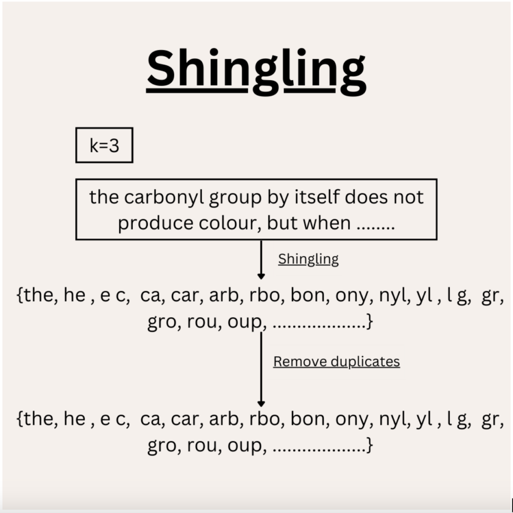
1. Shingling :
Shingling is a method of creating tokens of length k. The tokens are created by the following process : take the first k elements from a text [0:k-1], then skip the first element and take the next k tokens [1:k], then [2:k+1] and so on.
Here is a visual demonstration of Shingling :
After shingling is performed, the tokens would need to be converted to one-hot encoding. A vocabulary vector (which contains all the possible combinations of tokens of length k) is used. Another vector (let’s call it one-hot vector) with ‘0’ values is created, the size of this vector is equal to the size of the vocabulary. If the token is present in our shingles list, it is marked as 1 in the one-hot vector.
2. MinHashing
As one-hot encoded vectors can be huge and can take a lot of computations, convert one-hot encoded vectors into a dense vector. MinHashing is used for the conversion. If a dense vector of size ‘n’ is needed, Minhashing is applied ‘n’ times to the input sparse vector. In order to apply Minhashing, the contents of the sparse vector are shuffled and then the first vector position where a non-zero value is found is taken.
Here is a visual representation :
3. LSH Hashing :
The dense vector is hashed using a number(k) of hash functions, the results of the hash are stored in hash buckets for each function. One thing to keep in mind, hash collisions are encouraged in LSH, so that similar vectors can be stored in the same hash bucket.
In order to find similar vectors (which may not necessarily be entirely equal), if ‘j’(out of ‘k’ total hash functions) hash function outputs are matched, then the vectors are considered similar.
Here is a visual representation :
LSH are best for low-dimensional or small datasets.
Published by: Urvashi Poonia